In Part I of this series, we took a look at Messi’s role at Barcelona over his career, and developed a metric (xF – expected force) to demonstrate the magnitude of his impact at the club. In this post, we will shift our focus to outside Barcelona and towards the performances the two players who have dominated football for the last decade – Lionel Messi and Cristiano Ronaldo.
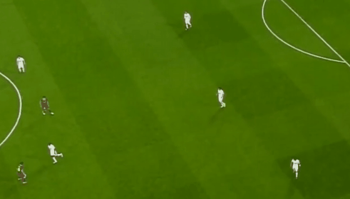
The most intriguing aspect of the Messi-Ronaldo comparison is how prolific both are in terms of goal scoring tallies, and yet how different both are in terms of playing style. Messi is often hailed as a “naturally gifted” player who uses his tremendous ability on the ball to outmaneuver defenders, while Ronaldo is often viewed as a phenomenal athlete who takes advantage of his superior strength, speed and power to out run and out jump opposition. Now since these are both general “intuitive” observations of the players, why not analyze data from head-to-head matches between the two to develop a more precise understanding of what sets them apart as players and what their play styles actually are? How about we start with an action map of all the dribbles, passes and shots taken by either player during the match:

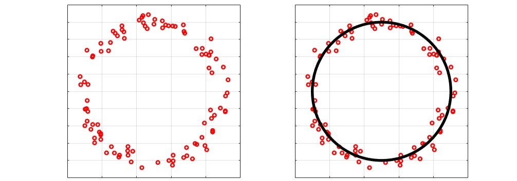
Now apart from the obvious that Ronaldo and Messi played off opposite wings, it’s hard to concretely identify a pattern for either player. More technically, what we want to try and find is a coherent structure within the distribution of points, just like how we can identify a “doughnut” in the ring of scattered points below:
So how could we go about finding such a structure? It turns out we can use tools from the mathematical field of topology to help us characterize features of the scattered event data for Messi and Ronaldo. In particular, we are going to use the method of persistent homology.
First, what is homology? To be technically correct, when we say homology, we’re actually referring to homology groups which is essentially a measure that counts the number of different dimensional “holes” in our structure, or equivalently the connectivity of our structure in different dimensions. For example, from the figure below we can see a 0-dimensional “hole” means disconnected parts in the structure (or the number of connected components), while a 1-dimensional hole could be a punctured disc in the plane (or the number of “rings” formed):

Before we get to finding holes though, we need an actual “surface” to analyze, and at the moment we only have a bunch of scattered points. To transform the latter into the former, we have to construct a simplicial complex; more specifically, we construct what’s called a Vietoris-Rips complex. What this means is we choose some distance r and we “connect” two points if the distance between them is less than r. A group of k points which are all mutually connected form a (k-1)-simplex, or a clique; so 2 connected points form a 1-simplex, 3 points form a 2-simplex and so on. The reason for having all points within a simplex being mutually connected is that we can then view all those points as a single unit, kind of like how a group of 11 players is 11 individuals but we can also just generally refer to the entire group as a single team. Ultimately, we can “fill” in the simplices to create the surface we wanted. The animations below show this process for increasing values of r:

OK, so now we have a way to generate surfaces to analyze, but how do we actually identify holes? Here’s where some knowledge of algebra will definitely be useful to follow some of the underlying mechanisms. The first step is to realize that the simplicial complex we created is just a set of simplices (the individual points, edges, triangles, tetrahedrons and so on which are formed by connecting points). Let’s call this set X. Then X contains all the different dimensional simplices in our complex and so we can denote all the k-dimensional simplices in X as the (sub)set Xk. Now to define another group called the chain group, Ck(X), which is essentially a rational vector space with a basis of Xk and represents all the k-dimensional chains. Let’s get a more geometric intuition of chain groups and hopefully start to see how they might be useful in our pursuit of finding “holes”; we’ll take a simplified simplicial complex like below and show some examples of elements in C1(X):
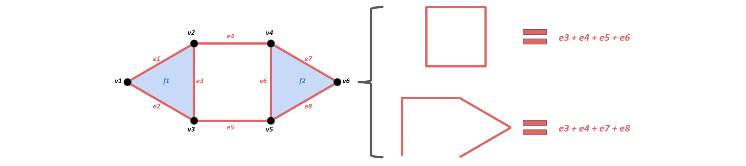
Now just by visual inspection, we can intuitively see that there’s a hole in our complex, right in the middle, composed of the sum of (e3+e4+e5+e6). Let’s rephrase this a bit: we see that the linear combination of (e3+e4+e5+e6) creates a path that is a “cycle” since it starts and ends at the same point. Finding these cycles seems like an important step towards finding holes so let’s create a linear map to help us do this, called the boundary operator (𝛿) defined as follows:
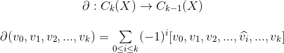
The first line is just a statement of the overall function of the operator; basically it takes k-dimensional chains and returns (k-1)-dimensional chains. So if we had a line (1-dimensional chain), the operator would return the boundary points of that line (points being 0-dimensional). The second line explains how this is done: the operator takes all the vertices (0…n) in the simplex, and returns an alternating sum of “sub”-simplices; that is, simplices with one vertex removed, which is what the carat on the v̂i is denoting — the simplex [v0,…,vk] with the vertex vi removed. Let’s try to gather an intuition about this using another example:

So the boundary operator on the triangle simplex returns to us the edges that “outline” the triangle. Put that way, it seems pretty simple but there’s actually a couple of other things going on here that get us pretty close to finally identifying the holes we’ve wanted all along. First, notice that the triangular boundary that was returned on the right is exactly like the path we had before with (e3+e4+e5+e6) in that it’s a cycle, but now we can see that these cycles actually occur every time the path sums to zero, or equivalently, every chain that gets mapped to 0 by the boundary operator is a cycle, OR in more algebraic terms, all the chains which are also cycles form a subgroup that is ker(𝛿k), the kernel of the boundary operator on the k-dimensional chain group.
The other thing that we should notice is that while we can now find all the cycles, that’s not the same as counting all the holes; looking at the two examples above, the triangle and the square form cycles, but the square actually formed a hole while the triangle was “filled in” by a face. So we need to distinguish the two and more importantly, a way to count only the cycles which don’t get filled in at a higher dimension. Terminology wise, we call cycles that bound a higher-dimensional face a boundary, and if the criteria for a chain cycle to be a boundary is that it gets filled in at a higher dimension, then why not see what our boundary operator returns at the next highest dimension? That is, what does 𝛿k+1 return? If it returns anything other than zero, then we can deduce from the logic above that the cycle has been filled in, that is the boundaries also form a subgroup that is im(𝛿k+1), the image of the boundary operator on the (k+1)-dimensional chain group.
Now that we can find all the cycles and all the boundaries, to find our “holes” we want to find all the cycles that aren’t boundaries. Formally, this is what’s called the k-dimensional homology group (Hk) which is a quotient space and we denote this as:

And then we can find the number of k-dimensional holes by computing the “size” or dimension of the k-th homology group which we can compute with:

Great. We’ve finally got to the point where given a simplicial complex we can find the holes in that complex, so that takes care of homology but what about persistence? Well going back to how we created the complex in the first place remember the first step was to choose a distance r which we used as a criteria to connect points; so how do we know which value of r to choose? The idea is that instead of choosing a single value of r we use a range of values, we compute the homology groups for each r and we take note of those holes which persist over a range of distance thresholds; we can consider those holes to be significant features of our data, while holes that appear but quickly close as r increases can be considered as “noise” or insignificant. Often we create a barcode plot to visualize this and we can see how one of these is produced below, using the example of finding 1-dimensional holes in Messi’s data:

Here on the x-axis is the distance r used to build the complex and the bars which are plotted represent the distances at which holes appear up to when holes are “covered”; the bars highlighted in red are the ones which have persisted for distances over a range of 2 meters. Essentially we see 3 significant holes appear around the range of r=15 meters. Let’s look at what the simplicial complex looks like for both Messi and Ronaldo using r=15, along with the barcode plots for 0-dimensional and 1-dimensional holes:

As mentioned with Messi, we see the 1-dimensional holes appear in his action map and with Ronaldo we don’t see any clear holes appear in his map. Instead, with Ronaldo we see that there seems to be several disconnected components, which we can also see in the 0-dimensional barcode plot. With Messi we see that components connect rather quickly, meaning they are quite clustered and this can also explain the 1-dimensional holes which appear; however, Ronaldo’s actions are quite dispersed which is why the 0-dimensional holes have such a slow drop off and no-significant 1-dimensional holes appear.
Now this was only a single match (from 2015), so how conclusive could it actually be? Well, let’s look at some other Clasicos from over the years:

So we see that the patterns we found in both Messi’s and Ronaldo’s play styles have also persisted over the years, and more interestingly how different they have always been as players despite the similarity in their goal and award tallies. But in a footballing context what might this mean? The holes in Messi’s map are quite literally groups of Madrid players, and represents how Messi slips around/through the midfield press, has a bit of freedom between the midfield and defensive lines before having to circumvent the Madrid’s defense again. Moreover, we see his reluctance to play into the corners of the pitch, instead cutting in onto his left foot and drifting into the center of the pitch well before the 18-yard box. By contrast, the void in Ronaldo’s map indicates his actions are typically split in two: either he is involved in some build-up play around the middle of the pitch or he is running onto through balls or crosses played into him in the final third. Otherwise his runs from midfield are far more direct compared to Messi, who mazes in and out of players.
I’ll end off this blog with clips from both players that really puts the analysis in context and highlights the difference in styles: